Project CETI
One of the leading research groups trying to unravel the communication between whales and humans is Project CETI. There are currently a couple of vessels in operation in Dominica conducting ongoing research via CETI’s custom-built bio-inspired equipment. Project CETI’s “Core Whale Listening Stations” represent a paradigm shift in animal communication monitoring, constituting the most advanced system ever devised for such a purpose and capable of capturing massive amounts of data for AI. This research facility is located off the coast of Dominica for initial testing and should be fully operational this fall/winter.
Why whales?
In many ways, whales behave similarly to human beings, which explains why they were chosen for this study. They have a complex form of communication, using echolocation pulse and clicks to converse. Furthermore, they have 26 types of “Codas”, which can be compared to dialects in the human language. They live in pods and families and have different cultures for different groups. Furthermore, their high residency rate offers a possibility for gathering a lot of information and now using machine learning and deep learning raises the potential of creating a “chatbot” for interspecies communication.
Study Design
The study is designed as follows:
Firstly, the raw data is captured. This is done by capturing the audio using underwater microphones. It is also important to contextualize the audio which is done using drones and small GPS trackers on the whales. and all this is being overseen by a watcher tower for better latency in communication.
Secondly, the data is cleaned and structured, which we will discuss later on in depth.
Then the language is extracted from the structured data.
Lastly and hopefully a sequence of codas should be synthesized and played back to the whales.
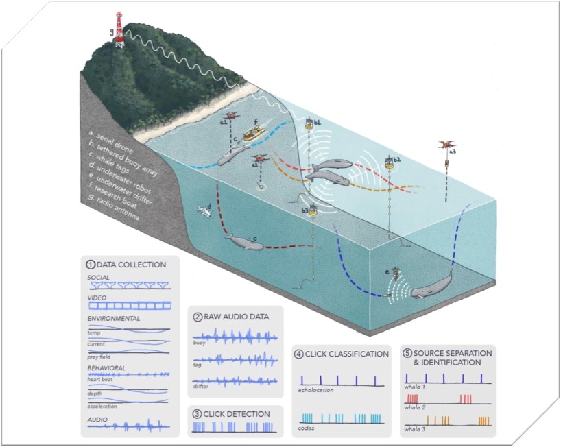 As we do not currently have implemented models from Project Ceti themselves, we will show similar deep-learning models, that should work the same way.
Detection
To collect data about the whales one has properly to distinguish whale sounds from the other ocean of sounds you get underwater. The program taking care of this crucial first step is Orca Spot.
Orca-Spot
ORCA-SPOT uses deep learning techniques, specifically convolutional neural networks (CNNs), that manage the binary classification problem: Whale sound or noise
ORCA-SPOT architecture is built upon the principles of a ResNet.
ResNet is a form of convolutional neural network largely used for image processing.
The developers chose ResNet 18 as a base design for the Orca Spot.
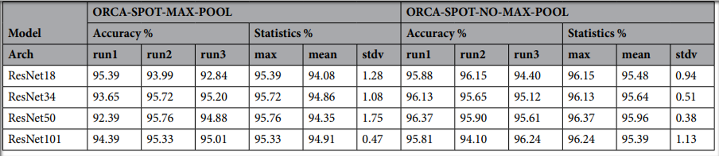
ResNet18 is the smallest and simplest among the ResNet variants. It proved to be a strong competitor due to its speed and efficiency. The ResNet18 architecture’s training and inference times were the shortest, making it a favorable option where real-time results are crucial. It can process 45-minute Orchive tape in 2 minutes Its accuracy was only about 0.5% less on average compared to the more complex ResNet50. Although ResNet34 has almost double the layers of Resnet18, it did not show any substantial improvement. Moreover, Resnet101 is the most complex among the ones tested and did not provide a significant boost in accuracy compared to its counterparts.
Architecture
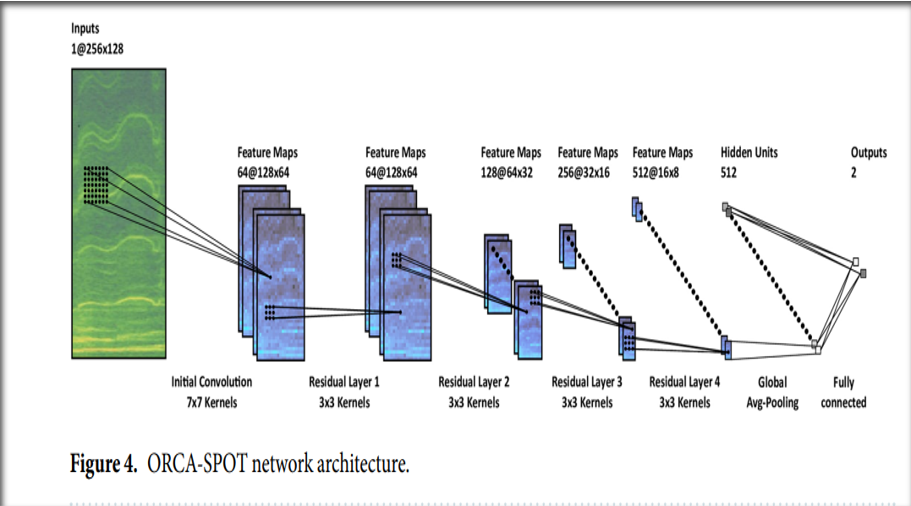 The developers of Orca-Spot modified the original ResNet design in specific ways to better handle its task of distinguishing killer whale sounds from noise.
For example, in traditional ResNet architecture, the max-pooling layer would cause a loss of resolution early in the network, which is unfavorable for handling high-frequency subtle killer whale signals. ORCA-SPOT circumvents this by keeping the resolution as high as possible for as long as possible, by removing max-pooling in the first residual layer.
The developers of Orca-Spot modified the original ResNet design in specific ways to better handle its task of distinguishing killer whale sounds from noise.
For example, in traditional ResNet architecture, the max-pooling layer would cause a loss of resolution early in the network, which is unfavorable for handling high-frequency subtle killer whale signals. ORCA-SPOT circumvents this by keeping the resolution as high as possible for as long as possible, by removing max-pooling in the first residual layer.
The second modification includes a global average pooling layer, in which it’s output is connected to a 512-D fully connected layer. Following that, this layer then overlays its result on the classifications “killer whale” and “noise,” providing the model’s final conclusion.
Training the model
In order to train the model, the audio clips were turned into 44.1kHz mono wav-signal and then converted into power spectrograms. To increase the variety of data the model trains on, intensity, pitch, time, and noise augmentation, were randomly scaled between two fixed ranges.
During the development and training of the Orca-Spot two models were created with different normalization approaches.
The Orca-Spot 2 model applies dB-normalization within a fixed range of 0–1, as a mean/standard deviation normalization approach in Orca-Spot 1 leads to high false-positive rates because when the standard deviation is close to zero in silent recordings, any small variation in the signal might be magnified by the normalization process, leading to extreme values and thereby higher false-positive rates.
Using dB-normalization (decibel normalization) the audio signal’s intensity (or loudness) is adjusted to fit within this specified range. In this case, the loudest signal is set as 1 and the quietest signal is set as 0, and everything else falls proportionally in-between, which helps avoid creating extreme values even if the original recording is very quiet.
Results
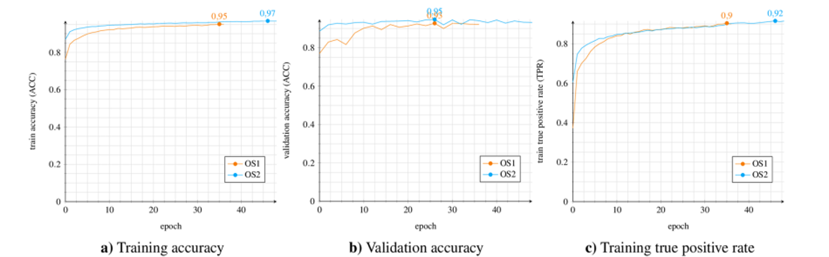 Both models were tested on 23,511 “Orchive” tapes.
Orca Spot 1 spotted 19,056 audio clips in which 16,646 segments were true killer whale sounds and 2,410 were falsely classified.
Orca Spot 2 spotted 19,211 audio clips, in which 17,451 segments were true killer whale sounds and 1,760 segments were falsely classified.
Both models were tested on 23,511 “Orchive” tapes.
Orca Spot 1 spotted 19,056 audio clips in which 16,646 segments were true killer whale sounds and 2,410 were falsely classified.
Orca Spot 2 spotted 19,211 audio clips, in which 17,451 segments were true killer whale sounds and 1,760 segments were falsely classified.
Orca-Clean
Thus far in the study, one of the main challenges was the underwater noise contamination i.e. boats … affecting data interpretation and feature learning. That’s where Orca-Clean comes in as a deep denoising network designed for denoising of killer whale underwater recordings. It doesn’t require any clean ground truth samples.
Preparation and training
Orca-Clean is prepared in a similar way as ORCA SPOT. The first stage of preparation involves converting audio signals into a form suitable for the experiment. Then synthetic and real-world underwater noises are added to challenge the denoising model and train it for an improvement in future results. In order to allow the network to focus on important areas within the spectrogram a Binary Mask Generation model was used. This process creates a ‘mask’ where it separates the audio into ‘spectrally strong’ and ‘spectrally weak’ signal regions for easier identification of useful areas in the spectrogram.
Network Architecture
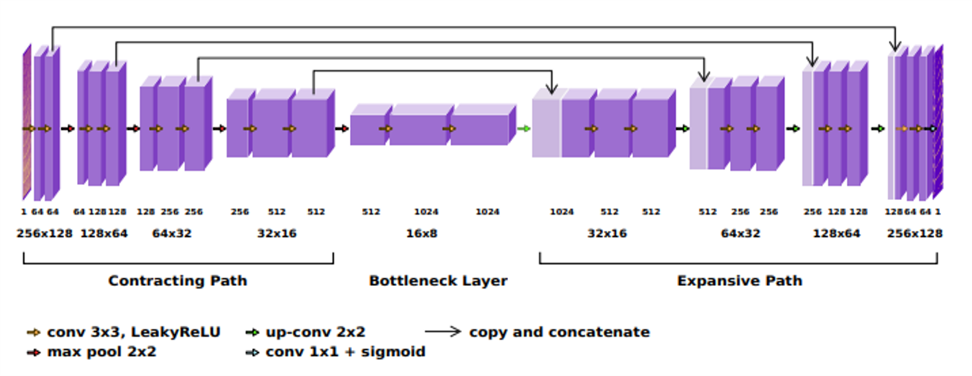
The experiment uses a deep learning model for denoising based on the U-Net architecture. Although U-Net is a well-known architecture for image segmentation tasks, in this instance, it has been customized for auditory information adaptation.
The Contracting, Bottleneck, and Expansive layers make up the three components of the U-Net architecture.
The Contracting (downsampling) path This route’s goal is to preserve the image’s context. It starts with a stack of convolutional layers—typically two—and then downsamples using a max-pooling process. The number of feature channels typically doubles with each downsampling step as we proceed along this path, enabling the network to learn more intricate features.
The bottleneck layer is situated between the Expansive and Contracting routes. The bottleneck layer serves as an extractor or summarizer of features.
The primary function of the bottleneck layer is to extract the input data’s most compact and abstract properties and then transfer this knowledge to the expanding path for use in the output reconstruction.
The expansive layer (upsampling) then makes use of this context to localize—also known as localization—the object in the image. The expansive approach uses a stack of convolutional layers, followed by an upsampling that boosts resolution and is almost a mirror image of the contracting path.
Results
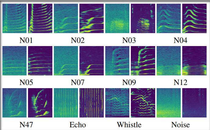
The accuracy represents the overall correctness of the system in identifying true positives and true negatives in the dataset. In this case, the system performs slightly better with Orca Clean improving the 94.97% accuracy to 96.04%. Precision is the proportion of true positive results among all the positive results predicted by the system. A higher precision indicates a lower number of false positives. The difference in precision, in this case, was very minimal but significant enough to drop the false-positive-rate from 4.36% to 1.77%
Classification
Orca-Feature
The Orca-Feature is a deep learning model that can classify and differentiate between different call types. This model can operate without the need for pre-existing labels or classifications. The pipeline is less prone to human error, as it offers a more objective approach when it analyses the sound, which eliminates human bias.
The structure of the model is somewhat close to the Orca-Spot and Orca-Clean. It is also a convolutional neural Network, that is based on ResNet18.
The model contains an under-complete autoencoder, that tries to accurately learn and reconstruct the input of the spectrogram image.
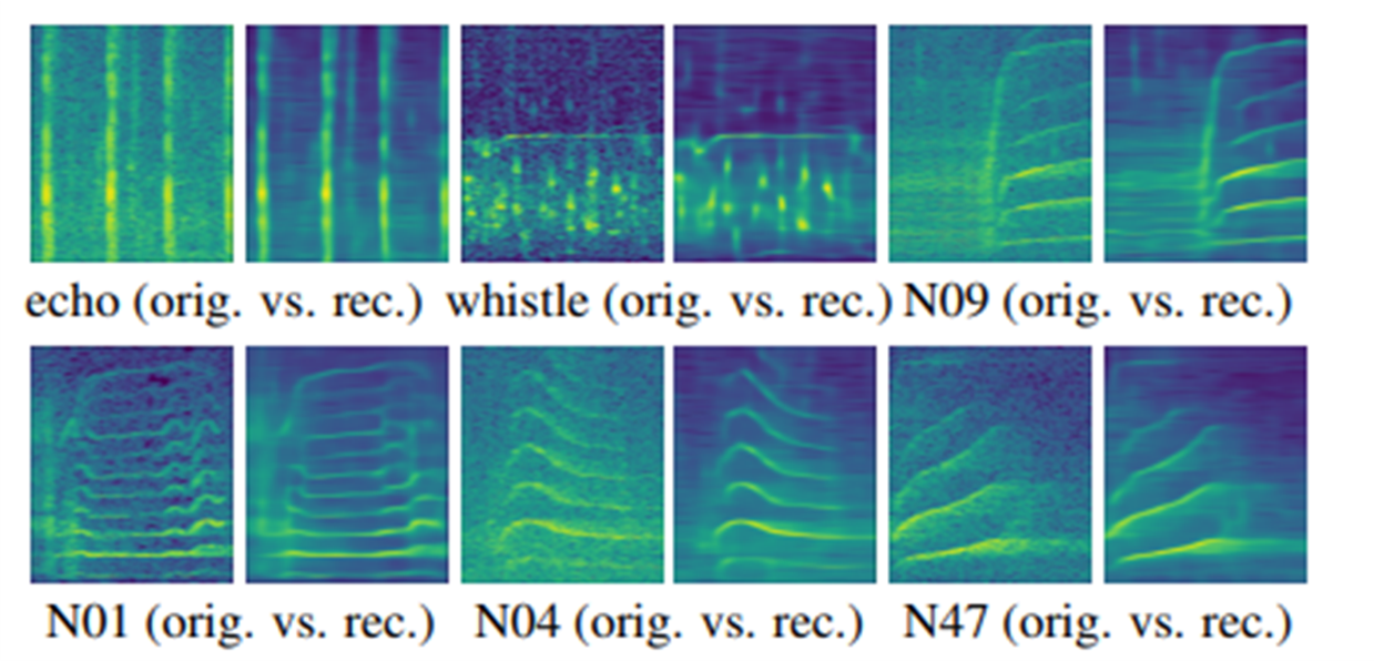
The autoencoder contains an encoder path, where it uses an encoder function on the input sample to get a hidden representation. Then a decoder path with a decoder function to reconstruct the original input. So, the main goal is to generate an output, that is as close as possible to the original input and that process enables Feature learning, which allows the model to understand important characteristics of each spectrogram image.
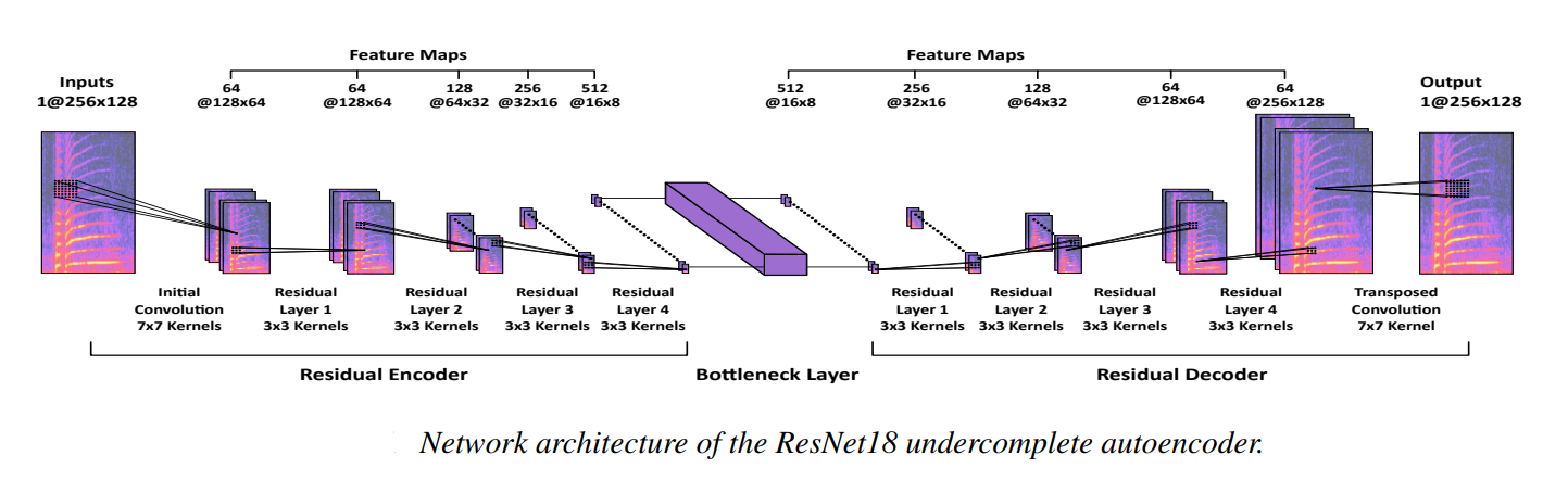
After the model learns the salient features of each spectrogram image, spectral clustering, an unsupervised learning technique, is used to group similar spectrogram images into 12 clusters on the basis of features together.
To Properly evaluate unsupervised Clustering, a comparison has been made to the supervised Classification model. This model has the same structure as Orca-Spot. However, the output is connected to a 12-D layer, to classify between 12 different call types, that have been trained to recognize.
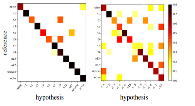
The confusion matrix clearly visualizes the comparison between the supervised(left) and unsupervised(right). The supervised classification reached around 85% accuracy, whereas, for the unsupervised model, there were a lot of misclassifications and reached around 60% accuracy. Nevertheless, does it mean the model was wrong?
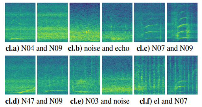
In the image above, for example in cluster C, we have two different spectrogram images, which the clustering algorithm grouped together, as they share the same features, thus viewing them as the same call type. However, humans classified them as different call types, specifically N07 and N09. This raises the question, did the humans misclassify them, or did the unsupervised clustering?
Orca-Slang
ORCA-SLANG is a machine-driven, multi-stage, semi-supervised, deep-learning framework for killer whale (Orcinus Orca) call type identification, designed for large-scale recognition of known call types and sub-call patterns and/or unlabeled vocalization categories.
Model Design
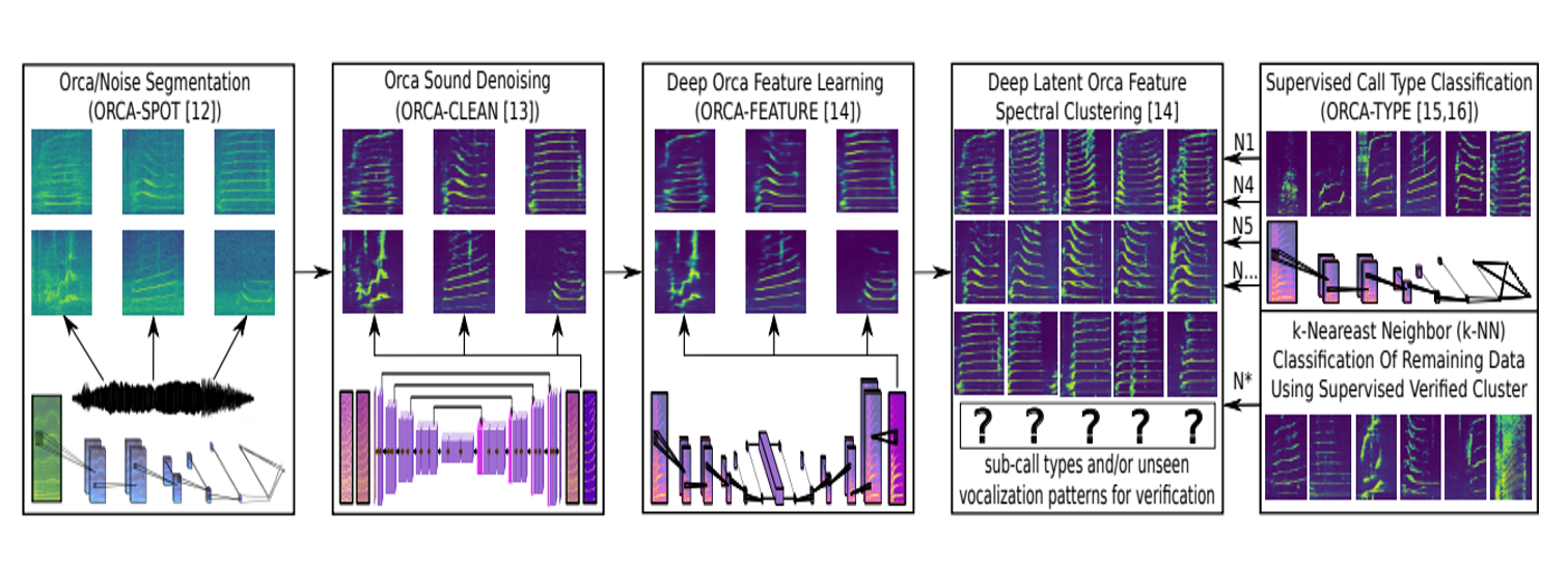 The Orca-Slang experimental setup uses a large database of audio samples called the ORCHIVE. This process occurs in four main steps:
- Segmentation with ORCA-SPOT as discussed before.
- Embedding and Enhancing with ORCA-CLEAN, where, the segmented recordings are enhanced, then
- ORCA-FEATURE using a machine learning training process with specific parameters (batch size, learning rate, etc.) and
- lastly Call Type Clustering and Classification with ORCA-TYPE and k-NN. This final step is a hybrid approach that involves both supervised and unsupervised learning. First, spectral clustering is performed on a random selection of 20,000 ORCA-SPOT segments, resulting in 200 clusters. Then, ORCA-TYPE is used to classify the content of all clusters to find those that belong to one of the nine trained call types. If more than 70% of a cluster is classified as a certain call type, it is grouped, summarized, and used to form a reference for the k-NN classification of all the remaining data excerpts. Clusters that don’t meet the 70% purity threshold are put in a rejection class. This final step is then repeated 5 times, removing duplicates, to ascertain the actual number of unique and additional detected call types across all trials The collaboration with k-NN classification reduces computational overhead and data storage needs.
K-Nearest Neighbour Algorithm
The k-nearest neighbors algorithm, sometimes referred to as KNN or k-NN, is a supervised learning classifier that employs proximity to produce classifications or predictions about the grouping of a single data point. In this study, the algorithm is only used for classification. A new data point is classified based on its similarity relative to all the existing data that has been stored. This means that by utilizing the K-NN method, fresh data can be quickly and accurately sorted into a suitable category.
Communication- Language Model
The identification of acoustic building blocks is necessary to construct a communication-language model. This involves identifying basic elements or phonetics in whale vocalizations by listening for patterns, such as vowels and consonants in human speech. Additionally, the grammatical structure must be determined, which entails figuring out the rules that control how these fundamental building blocks are arranged, similar to the syntax in human languages. Furthermore, in order to prevent building a “whale-chat bot” that can communicate with sperm whales but is not comprehensible to humans, the behavioral data must be linked with the codas. Presumably, a Language Model has not been implemented yet, however, a roadmap has been laid out. Project Ceti intends to use an unsupervised translation method such as the following example.
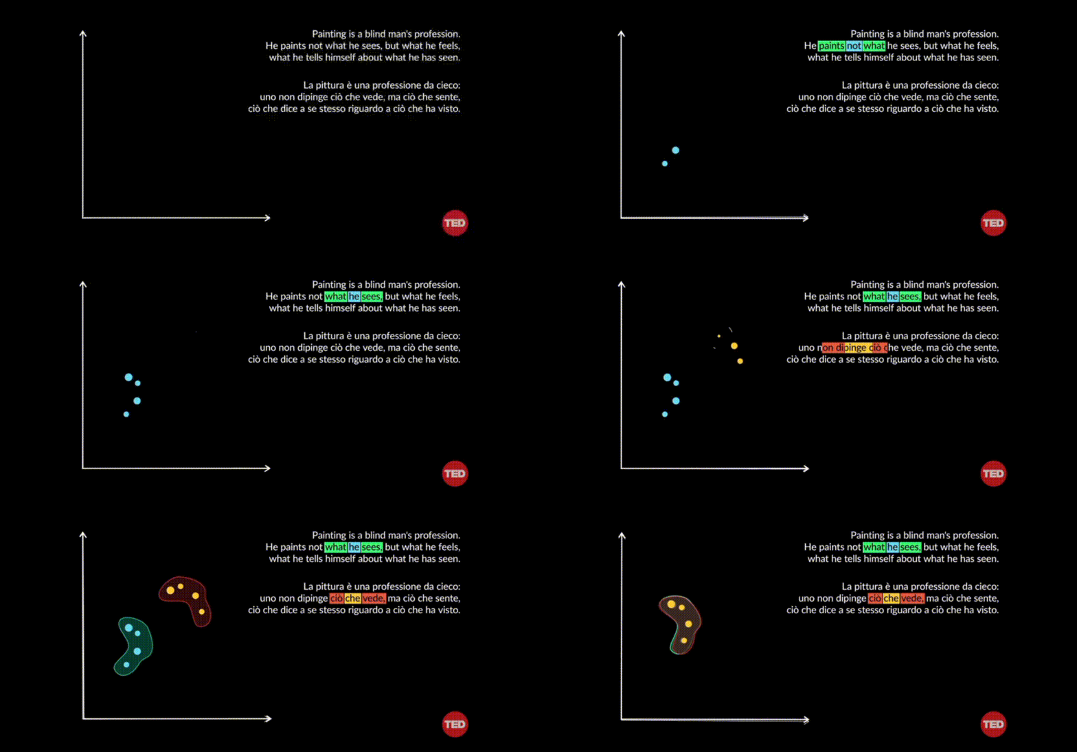 There are two different languages and each word generates through an encoder an embedding, which is a multidimensional vector representation. When these embeddings of different words are grouped together(sentence), they create a geometrical shape. The alignment of the two geometrical shapes suggests that there may be semantic similarities. With this unsupervised approach, an association can be determined from two different languages, directly from the embeddings. However, in order for this to operate, a remarkable amount of data is required. This includes but is not limited to codas, data regarding behavior, geographical location, and biological data.
Conclusion
After discussing the model of the study and observing the progress made one could conclude that the potential shown in this field seems to be promising. As fascinating and interesting as interspecies communication sounds there is still a lot of progress to be made. In theory, one could say that the goals are achievable in the foreseeable future but in real life, it may never go as planned. But what is known for sure is that through this research we will obtain new knowledge, and if this goal is not met, the acquired information will be used in other fields that will benefit the scientific community.